The Basics of Mean Reversion
11 Apr 2022Most price series are not mean reverting, but are geometric random walks. The returns, not the prices, are the ones that usually random distribute around a mean of zero. Unfortunately we cannot trade around the mean reversion of returns. One must not confuse mean reversion of returns with anti-serial-correlation of returns which we can definitely trade one. But anti-serial correlation of returns is the same as mean reversion of prices.
Most price series are not mean reverting. Fortunately, we can manufacture many more mean-reverting price series than thre are traded assets because we can often combine two or more individual price series that are not mean reverting into a portfolio whose net markets value (price) is mean reverting. Time series which can be combined this way are called cointegrating. There are statistical test to spot this, the CADF and Johansen test (gives us the exact weightings of each asset to create a cointegrating portfolio).
Mean reversion and stationarity are two equivalent ways of looking at the same type of price series, but these two ways give rise to two different statistical tests.
Mean reverting time series:
- the change of the price series in the next period is proportional to the difference between the mean price and the current price
- this gives rise to the ADF test, we tests if the proportionality constant ($\lambda$) is zero
Stationary time series:
- mathematically stationary time series imply that variance of the log of the prices increases slower than that of a geometric random walk (variance is a sublinear function of time instead of linear)
- the sublinear function is approximated by $\tau^{2H}$, where $\tau$ is time and H is called the Hurst-exponent. The Variance ratio test checks if the exponent is actually 0.5
ADF Test
We describe the price changes of a linear model as follow :
\[\Delta y(t)=\lambda y(t-1) + \mu+ \beta t + \alpha_1\Delta y(t-1) + \dots + \alpha_k\Delta y(t-k) + \epsilon_t\]the ADF checks if the $\lambda$=0 (null hypothesis). If the hypothesis can be rejected this means that the next move depends on the current level, and therefore it is not a random walk. Since we expect mean reversion $\lambda$ has to be negative.
Notes
- We assume that the drift is $\beta=0$ because it tends to be much smaller than the daily fluctuations in price
- Sampling data at intraday frequency will not increase the statistical significance of our test
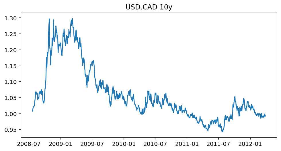
Example USD.CAD
from statsmodels.tsa.stattools import adfuller

data = yf.download("USDCAD=X", start="2008-07-22", end="2012-03-28")
x = data['Close'].values
result = adfuller(x, maxlag=1)
# Show results
print('ADF Statistic: %f' % result[0])
print('p-value: %f' % result[1])
print('Critical Values:')
for key, value in result[4].items():
    print('\t%s: %.3f' % (key, value))
ADF Statistic: -1.597062
p-value: 0.485069
Critical Values:
  1%: -3.437
  5%: -2.865
  10%: -2.568
We fail to reject the null hyopthesis at the 90% level, thus our time series is not mean reverting. Lambda was negative so at least we can say it is not trending.
Hurst Exponent and Variance Ratio Test
Intuitively a “stationary” price series means that the price diffuses from its initial value more slowly than a geometric random walk. Mathematically we can define this as:
\[Var(\tau)=\langle|z(t+\tau)-z(t)|^2\rangle\sim\tau\]the variance is proportional to $\tau$ for geometric random walks. However if the price series is trending or mean reverting then this equation will not hold. Instead, we can write:
\[\langle|z(t+\tau)-z(t)|^2\rangle\sim\tau^{2H}\]for a price series exhibiting a geometric random walk, $H=0.5$. But for a mean-reverting series, $H<0.5$, and for a trending series, $H>0.5$. $H$ serves also as an indicator for the degree of mean reversion of trendiness. $H$ towards zero means more mean reverting and $H$ towards 1 the series is trending more.
To test statistical significance we perform the variance ratio test, which checks if the following is equal to 1.
\[\frac{Var(z(t)-z(t-\tau)}{\tau Var(z(t)-z(t-1))}\]Code from taken from here
def hurst(ts):
    """
    Returns the Hurst Exponent of the time series vector ts

    Parameters
    ----------
    ts : `numpy.array`
        Time series upon which the Hurst Exponent will be calculated

    Returns
    -------
    'float'
        The Hurst Exponent from the poly fit output
    """
    # Create the range of lag values
    lags = range(2, 100)

    # Calculate the array of the variances of the lagged differences
    tau = [np.sqrt(np.std(np.subtract(ts[lag:], ts[:-lag]))) for lag in lags]

    # Use a linear fit to estimate the Hurst Exponent
    poly = np.polyfit(np.log(lags), np.log(tau), 1)

    # Return the Hurst exponent from the polyfit output
    return poly[0]*2.0
hurst(x)
0.43934474544953883
def variance_ratio(ts, lag = 2):
    """
    Returns the variance ratio test result
    """
    # Apply the formula to calculate the test
    n = len(ts)
    mu  = sum(ts[1:n]-ts[:n-1])/n;
    m=(n-lag+1)*(1-lag/n);
    b=sum(np.square(ts[1:n]-ts[:n-1]-mu))/(n-1)
    t=sum(np.square(ts[lag:n]-ts[:n-lag]-lag*mu))/m
    return t/(lag*b)
variance_ratio(x)
1.0259343090759017
Half-Life of Mean Reversion
In trading we can be can often be profitable even without the requirements of 90% certainty. A key observation is our interpretation of $\lambda$ as a measure of how long it takes for a price to mean revert. We can rewrite the ADF test linear formula in its inifitesimal form (ignoring the drift term). This yields the Ornstei-Uhlenbeck formula for mean-reverting process:
\[dy(t)=(\lambda y(t-1)+\mu)dt + d\epsilon\]where now we can take the expected value of this random process, yielding:
\[E(y(t))=y_0exp(\lambda t)-\frac{\mu}{\lambda}(1-exp(\lambda t))\]remebering that $\lambda$ is negative, this tells us that the expected value of the price decays exponentially to the value $\frac{\mu}{\lambda}$ with the half life decay equals to $\frac{-log(2)}{\lambda}$.
Notes
- If $\lambda$ is positive the price series is not mean reverting so don’t attempt a mean-reverting strat at all
- $\lambda$ close to zero means a very long half-life, therfore it is going to take a long time to converge to the mean thus it is not very profitable
- $\lambda$ determines many parameters in our trading strategy. For example if the half life is 20 days we should use a 20 day moving average as a parameter, or a multiple close to 20
Example on USD.CAD
We regress $y(t)-y(t-1)$ on $y(t-1)$ to find $\lambda$ and compute the half life $\frac{-log(2)}{\lambda}$
import statsmodels.api as sm

delta = data['Close'] - data['Close'].shift(1)
Y = delta.dropna()
X = data['Close'].shift(1).dropna()
X = sm.add_constant(X)
model = sm.OLS(Y,X)
results = model.fit()
                            OLS Regression Results
==============================================================================
Dep. Variable:                  Close   R-squared:                       0.003
Model:                            OLS   Adj. R-squared:                  0.002
Method:                 Least Squares   F-statistic:                     2.551
Date:                Mon, 11 Apr 2022   Prob (F-statistic):              0.111
Time:                        16:42:22   Log-Likelihood:                 3168.6
No. Observations:                 960   AIC:                            -6333.
Df Residuals:                     958   BIC:                            -6323.
Df Model:                           1
Covariance Type:            nonrobust
==============================================================================
                 coef    std err          t      P>|t|      [0.025      0.975]
------------------------------------------------------------------------------
const          0.0057      0.004      1.588      0.113      -0.001       0.013
Close         -0.0054      0.003     -1.597      0.111      -0.012       0.001
==============================================================================
Omnibus:                       87.993   Durbin-Watson:                   1.946
Prob(Omnibus):                  0.000   Jarque-Bera (JB):              331.047
Skew:                           0.365   Prob(JB):                     1.30e-72
Kurtosis:                       5.783   Cond. No.                         25.0
==============================================================================

Notes:
[1] Standard Errors assume that the covariance matrix of the errors is correctly specified.
halflife = int(-np.log(2)/results.params[1])
print(f"Half-life of mean reversion: {halflife} days")
Half-life of mean reversion: 128 days
A Linear Mean-Reverting Trading Strategy
Once we have determined a price series is mean reverting a simple trading strategy can be the following: determine the normalized deviation of the price (moving standard deviation divided by the moving standard deviation of the price) from its moving average, and maintain the number of units in this asset negatively proportional to this normalized deviation.
movingAvg = data['Close'].rolling(halflife).mean()
movingStd = data['Close'].rolling(halflife).std()
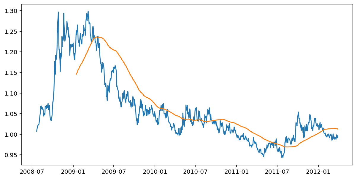
y = data['Close']
mktVal = -(y-movingAvg)/movingStd
pnl = mktVal.shift(1)*(y-y.shift(1))/y.shift(1)
Cointegration
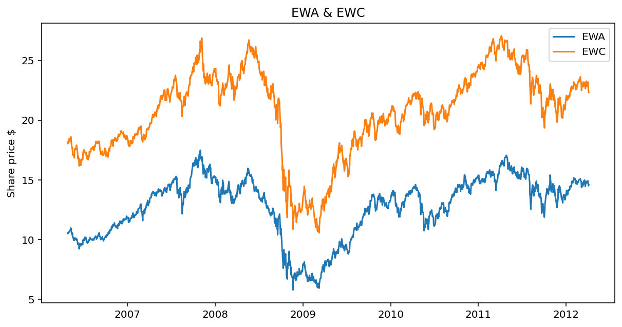
We are not confined to “prefabiacted” fianancial price series: we can proactively create a portfolio of individual price series so that the market value (or price) series of this portfolio is stationary. This is the notion of cointegration: can we find a a stationary linear combination of several nonstationary price series, if so then these price series are cointegrating. The most common example is that of two prices: we are long one asset and short another asset, this is pairs trading.
Cointegrated-ADF
The test first runs a linear regression between the two price series to find the hedge ratio. We then construct a portfolio of the two assets use the ADF test to check for stationarity.
Example EWA & EWC
ewa = yf.download("EWA", start="2006-04-26", end="2012-04-09")
ewc = yf.download("EWC", start="2006-04-26", end="2012-04-09")
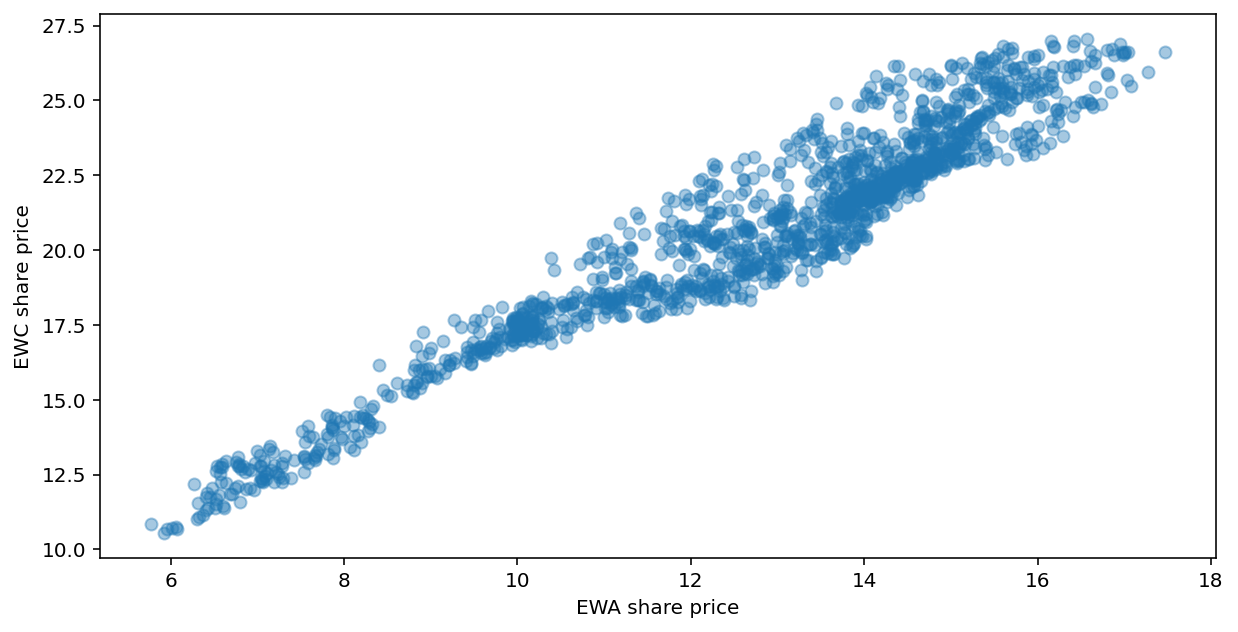
X = sm.add_constant(x)
model = sm.OLS(y,X)
results = model.fit()
hedgeRatio = results.params[1]
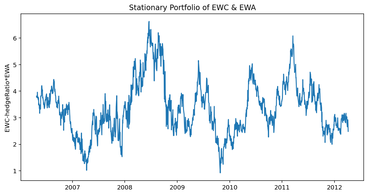
portfolio = y-hedgeRatio*x # the stationary porfolio

result = adfuller(portfolio, maxlag=1)
# Show results
print('ADF Statistic: %f' % result[0])
print('p-value: %f' % result[1])
print('Critical Values:')
for key, value in result[4].items():
    print('\t%s: %.3f' % (key, value))
ADF Statistic: -3.644006
p-value: 0.004973
Critical Values:
	1%: -3.435
	5%: -2.863
	10%: -2.568
Johansen
We first generalize the AR(1) equation to vectors:
\[\Delta Y(t)=\Lambda Y(t-1) + M + \epsilon_t\]we compute the rank of matrix the $\Lambda$ and check wether we can reject the null hypthesis that $r=0, r\leq1,\cdots, r\leq n-1$. If all these hypotheses are rejected, then clearly $r=n$ and we can form a stationary portoflio using all the assets. A useful by product is that the eigenvector associated with the biggest eigenvalue will give us the hedge ratios for our portofolio with the smallest half-life.
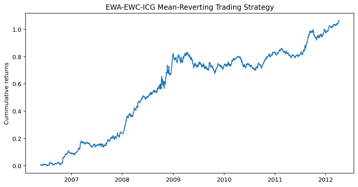
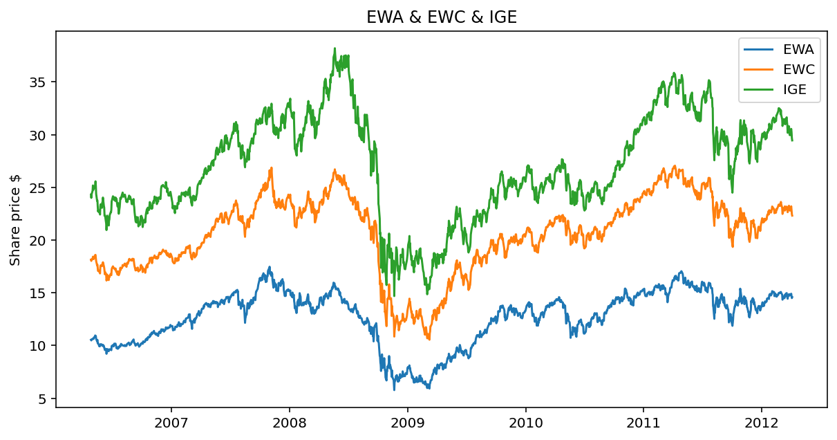
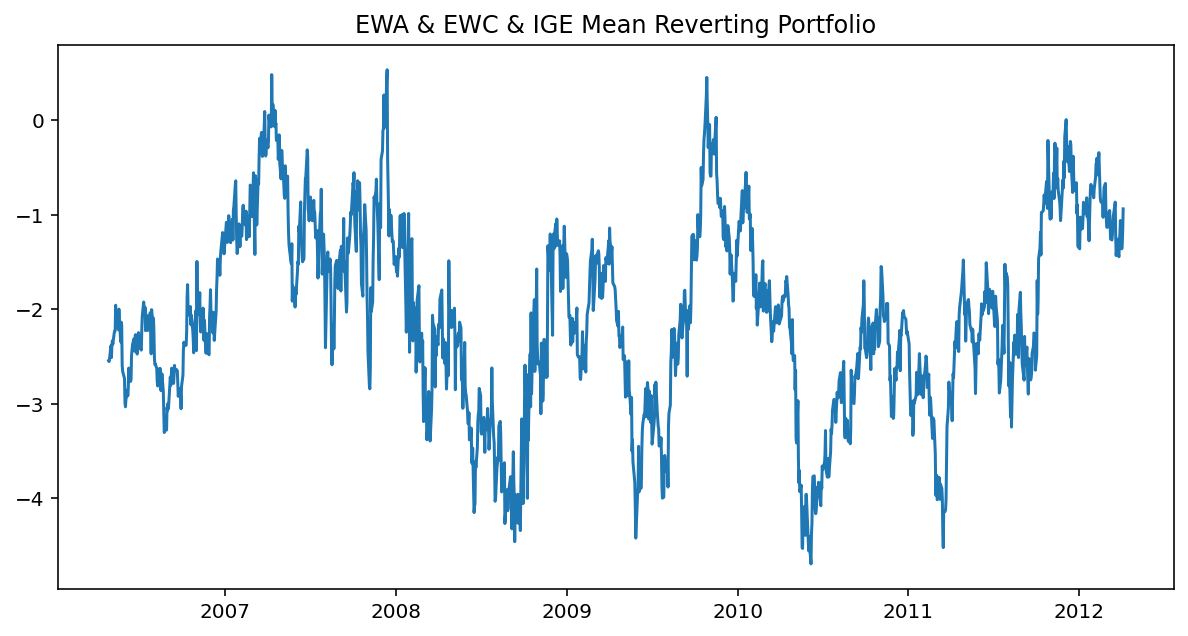
Example EWC-EWA-ICE
from statsmodels.tsa.vector_ar.vecm import coint_johansen

ige = yf.download("IGE", start="2006-04-26", end="2012-04-09") # natural resource stock ETF
z = ige["Adj Close"]

y3 = pd.concat([x,y,z], axis=1)
res = coint_johansen(y3,0,1)
joh_output(res)
   max_eig_stat  trace_stat
0     17.804192   34.637385
1     12.446337   16.833193
2      4.386856    4.386856

Critical values(90%, 95%, 99%) of max_eig_stat
 [[18.8928 21.1314 25.865 ]
 [12.2971 14.2639 18.52  ]
 [ 2.7055  3.8415  6.6349]]

Critical values(90%, 95%, 99%) of trace_stat
 [[27.0669 29.7961 35.4628]
 [13.4294 15.4943 19.9349]
 [ 2.7055  3.8415  6.6349]]
hedge_ratios = res.evec[:,0]
yport = y3*hedge_ratios # dot product between ETFs and hedge ratios
yport = yport.sum(axis=1)
ylag = yport.shift(1)

deltaY = yport-ylag
deltaY = deltaY.dropna()

ylag = ylag.dropna()
ylag = sm.add_constant(ylag)

model = sm.OLS(deltaY,ylag)
regress_results = model.fit()
halflife = -np.log(2)/regress_results.params[0]
print(f"Halflife: {int(halflife)} days")
Halflife: 21 days
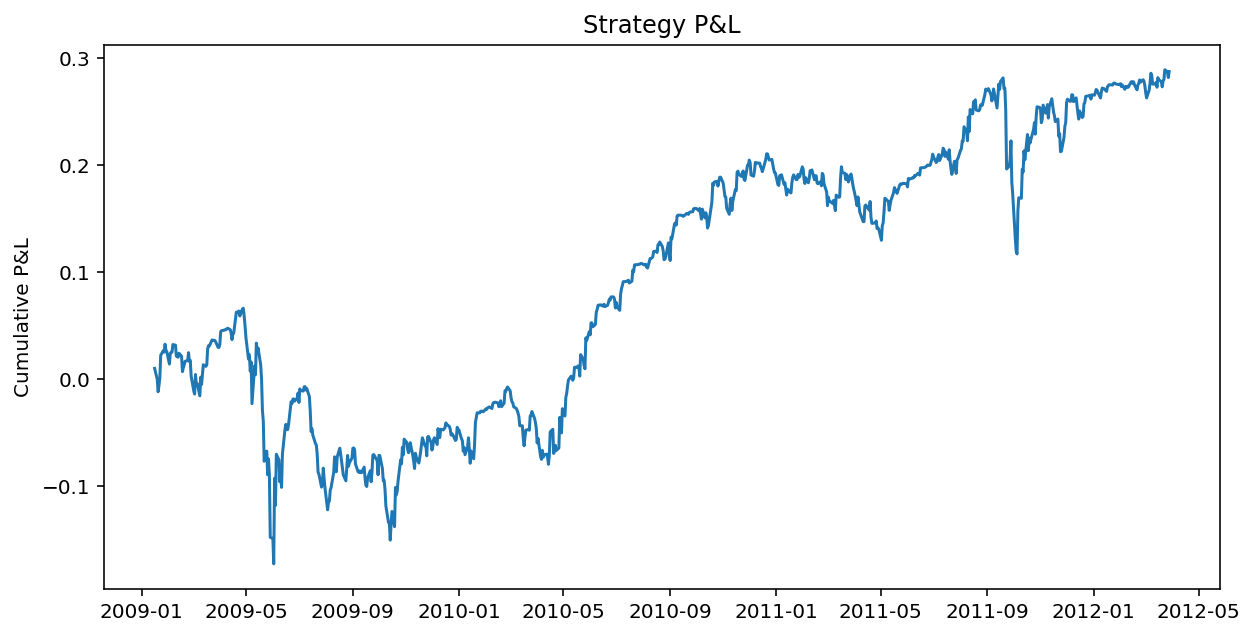
Linear Mean-Reverting Trading on a Portfolio
lookback = int(halflife)
numUnits = -(yport-yport.rolling(lookback).mean())/yport.rolling(lookback).std() # units of the stationary portfolio
# $ value of each ETF we own scaled by the units of the overall portfolio
positions = y3*hedge_ratios
positions.iloc[:,0] = positions.iloc[:,0]*numUnits
positions.iloc[:,1] = positions.iloc[:,1]*numUnits
positions.iloc[:,2] = positions.iloc[:,2]*numUnits
# pnl of the strategy
inter = positions.shift(1) * (y3-y3.shift(1))/y3.shift(1)
pnl = inter.sum(axis=1)
# daily returns of the strategy
ret = pnl/abs(positions.shift(1)).sum(axis=1)